The permimp-package

Dries Debeer

University of Zurich

2025-03-28

Abstract

The permimp-package is developed to replace the Conditional Permutation Importance (CPI) computation by the varimp-function(s) of the party-package. permimp applies a different implementation for the CPI, in order to mitigate some issues related to the implementation of the CPI in the party-package. In addition, the CPI is also available for random forests grown by the randomForest-package. Finally, the package includes some plotting options.

---

Introduction

Although originally designed for prediction purposes, Random forests Breiman (2001) have become a popular tool to assess the importance of predictors. Several methods and measures have been proposed, one of the most popular ones is the Permutation Importance Breiman (2001), originally referred to as the Mean Decrease in Accuracy. Inspired by the contrast between the unconditional zero-order correlation between predictor and outcome, and the conditional standardized regression coefficient in multiple linear regression, Strobl et al. (2008) argued that in some cases the importance of a predictor, conditionally on (all) other predictors, may be of higher interest than the unconditional importance. Therefore, they proposed the Conditional Permutation Importance, which introduces a conditional permutation scheme that is based on the dependence between the predictors.

The permimp-package presents a different implementation of this Conditional Permutation Importance. Unlike the original implementation (available in the party R-package of Hothorn, Hornik, and Zeileis (2006)), permimp can, in addition to random forests that were grown according to the unbiased recursive partitioning (cf. cforests; Hothorn, Hornik, and Zeileis (2006)), also deal with with random forests that were grown using the randomForest-package Liaw and Wiener (2002), which applies the original tree growing algorithm based on impurity reduction Breiman (2001). (In principle, the permimp can be extended to random forests grown by other packages, under the condition that tree-wise predictions are possible and OOB-information as well as the split points are available per tree.) We argue that the permimp-package can be seen as a replacement for the varimp-functions of the party package in R.

This vignette has two main parts. The first part is tutorial-like and demonstrates functionality of the permimp-package (by also comparing it to original party::varimp-functions. The second part is more theoretical and explains the how and the why of the new Conditional Permutation Importance-implementation.

Part I: permimp-tutorial

A. The permimp-function

The permimp-function replaces all the party::varimp-functions (varimp, varimpAUC, varimpsurv). To apply permimp-function, one needs a fitted random forest. Within this tutorial we will mainly focus on random forests-objects as obtained by the party::cforest-function (i.e., S4-objects of class "RandomForest"). As an example we will use the (cleaned) airquality-data set to fit random forest with 50 trees:

library("party", quietly = TRUE)
#> 
#> Attaching package: 'zoo'
#> The following objects are masked from 'package:base':
#> 
#>     as.Date, as.Date.numeric
library("permimp")
set.seed(542863)
airq <- subset(airquality, !(is.na(Ozone) | is.na(Solar.R)))
cfAirq50 <- cforest(Ozone ~ ., data = airq,
                    control = cforest_unbiased(mtry = 2, ntree = 50,
                                              minbucket = 5, 
                                              minsplit = 10))

A.1. New Conditional Permutation Importance

Let’s start by comparing the permimp and the varimp function for the conditional permutation importance.

system.time(CPI_permimp <- permimp(cfAirq50, conditional = TRUE, progressBar = FALSE))
#>    user  system elapsed 
#>   0.183   0.011   0.194
system.time(CPI_varimp <- varimp(cfAirq50, conditional = TRUE))
#>    user  system elapsed 
#>   1.285   0.011   1.296
CPI_permimp
#>    Solar.R       Wind       Temp      Month        Day 
#>  83.736656 209.786231 422.671385   1.820496  -7.668462
CPI_varimp
#>    Solar.R       Wind       Temp      Month        Day 
#>  25.147792 114.250197 220.080351   1.952776  -1.265111

Three differences can easily be spotted:

• permimp has a progressBar-argument. The default is progressBar = interactive()¹
• permimp is faster than varimp.
• The results are different.

A.2. Different results?

Why are the results different?

There are two main reasons.

First, permimp uses a different default threshold-value: permimp uses threshold = .95 while varimp uses threshold = 0.2. Check ?permimp and ?varimp. There is a good reason for using a higher default threshold value.

When using equal threshold-values…

CPI_permimp <- permimp(cfAirq50, conditional = TRUE, threshold = .2, progressBar = FALSE)
CPI_permimp
#>     Solar.R        Wind        Temp       Month         Day 
#>  26.9974775 122.2781497 204.0238116  -3.1201748   0.8442593
CPI_varimp
#>    Solar.R       Wind       Temp      Month        Day 
#>  25.147792 114.250197 220.080351   1.952776  -1.265111

The results are more similar, but not quite identical. The remaining differences are explained by the second reason: the implementation of permimp differs from the varimp-implementation. Using a higher threshold-value makes the differences between the two implementations more pronounced.

CPI_varimp <- varimp(cfAirq50, conditional = TRUE, threshold = .95)
CPI_permimp
#>     Solar.R        Wind        Temp       Month         Day 
#>  26.9974775 122.2781497 204.0238116  -3.1201748   0.8442593
CPI_varimp
#>    Solar.R       Wind       Temp      Month        Day 
#>  36.758973 198.610059 257.916926  -2.537016  -2.530303

The differences between the two implementations (and why we believe the new implementation is more attractive), is explained in the second part of this document, as well as in this manuscript: Debeer and Strobl (2020).

A.3. Backward Compatible with party when: asParty = TRUE

By specifying asParty = TRUE, the permimp-function can be made backward compatible with the party::varimp-function. But permimp is a bit faster. To get exactly the same results, the random seeds should be exactly the same.

set.seed(542863)
system.time(CPI_asParty <- permimp(cfAirq50, conditional = TRUE, asParty = TRUE, progressBar = FALSE))
#>    user  system elapsed 
#>   0.262   0.000   0.263
set.seed(542863)
system.time(CPI_varimp <- varimp(cfAirq50, conditional = TRUE))
#>    user  system elapsed 
#>   1.266   0.000   1.266
CPI_asParty
#>    Solar.R       Wind       Temp      Month        Day 
#>  36.364271 136.732886 200.620728   3.179600   1.360632
CPI_varimp
#>    Solar.R       Wind       Temp      Month        Day 
#>  36.364271 136.732886 200.620728   3.179600   1.360632

Note that with asParty = TRUE the default threshold-value is automatically set back to 0.2.

A.4. Different Output: VarImp-object

A less obvious difference between permimp and varimp is the object that it returns. permimp returns an S3-class object: VarImp, rather than a named numerical vector. A VarImp object is a named list with four elements:

1. $values: holds the computed variable importance values.
2. $perTree: holds the variable importance values per tree (averaged over the permutations when nperm > 1).
3. $type: the type of variable importance.
4. $info: other relevant information about the variable importance, such as the used threshold.

## varimp returns a named numerical vector.
str(CPI_varimp)
#>  Named num [1:5] 36.36 136.73 200.62 3.18 1.36
#>  - attr(*, "names")= chr [1:5] "Solar.R" "Wind" "Temp" "Month" ...

## permimp returns a VarImp-object.
str(CPI_asParty)
#> List of 4
#>  $ values : Named num [1:5] 36.36 136.73 200.62 3.18 1.36
#>   ..- attr(*, "names")= chr [1:5] "Solar.R" "Wind" "Temp" "Month" ...
#>  $ perTree:'data.frame': 50 obs. of  5 variables:
#>   ..$ Solar.R: num [1:50] 117.35 0 1.81 0 58.22 ...
#>   ..$ Wind   : num [1:50] 118.8 430.7 141.5 171 78.1 ...
#>   ..$ Temp   : num [1:50] 374 433 118 -1 175 ...
#>   ..$ Month  : num [1:50] -4.59 0 34.93 -11.96 -11.9 ...
#>   ..$ Day    : num [1:50] 0 18.93 0 7.18 0 ...
#>  $ type   : chr "Conditional Permutation"
#>  $ info   :List of 4
#>   ..$ threshold   : num 0.2
#>   ..$ conditioning: chr "as party"
#>   ..$ outcomeType : chr "regression"
#>   ..$ errorType   : chr "MSE"
#>  - attr(*, "class")= chr "VarImp"

## the results of permimp(asParty = TRUE) and varimp() are exactly the same.
all(CPI_asParty$values == CPI_varimp)
#> [1] TRUE

An advantage of the VarImp-object, is that the $perTree-values can be used to inspect the distribution of the importance values across the trees in a forest. For instance, the plotting function (demonstrated below) can be used to visualize this distribution of per tree importance values.

A.5. Unconditional Permutation Importance: permimp = varimp

Of course, there is also the option to compute the unconditional permutation importance. Both using the original and the split wise permutation algorithm. Here, there are no differences between permimp and varimp. That is, permimp simply uses the party varimp code, making the asParty argument redundant in this case. Note, however, that permimp still returns a VarImp-object.

## Original Unconditional Permutation Importance
set.seed(542863)
PI_permimp <- permimp(cfAirq50, progressBar = FALSE, pre1.0_0 = TRUE)
set.seed(542863)
PI_varimp <- varimp(cfAirq50, pre1.0_0 = TRUE)
PI_permimp
#>      Solar.R         Wind         Temp        Month          Day 
#> 104.19612764 345.36320352 582.09815801  18.04859049   0.01880503
PI_varimp
#>      Solar.R         Wind         Temp        Month          Day 
#> 104.19612764 345.36320352 582.09815801  18.04859049   0.01880503

## Splitwise Unconditional Permutation Importance
set.seed(542863)
PI_permimp2 <- permimp(cfAirq50, progressBar = FALSE, oldSeedSelection = TRUE)
set.seed(542863)
PI_varimp2 <- varimp(cfAirq50)
PI_permimp2
#>    Solar.R       Wind       Temp      Month        Day 
#>  81.935250 451.459770 580.918085  21.851431  -4.613963
PI_varimp2
#>    Solar.R       Wind       Temp      Month        Day 
#>  81.935250 451.459770 580.918085  21.851431  -4.613963

Note that the argument oldSeedSelection = TRUE was added when using permimp. Since the release of version 1.1-0, the way random seeds are used has been changed. Choosing oldSeedSelection = TRUE makes the computations backward compatible with older releases. However, when using parallel processing the old selection of random seeds holds problems for reproducible results. Hence, it is recommend to use the default oldSeedSelection = FALSE, especially when using parallel processing.

For more detailed information check ?permimp.

B. Methods for VarImp-objects

B.1. plot

Visualizing the variable importance values (as a VarImp-object) is easy using the plot method. Its main features include:

• Four plot types:`type = c(“bar”, “box”, “dot”, “rank”).
• Predictors automatically ordered according to importance value (high to low). Setting the argument sort = FALSE renders the original order (cf. the cforest call).
• with argument horizontal = TRUE horizontal plots are made.
• Optional visualization of the $perTree importance value distribution with the interval argument. With type = "box", the distribution of the $perTree-values is automatically visualized.²

We would suggest to only use the visualization of the $perTree importance value distribution, when there are enough trees (>= 500) in the random forest. Therefore, we first fit a new, bigger random forest, and compute the permutation importance.

## fit a new forest with 500 trees
set.seed(542863)
cfAirq500 <- cforest(Ozone ~ ., data = airq,
                     control = cforest_unbiased(mtry = 2, ntree = 500,
                                              minbucket = 5, 
                                              minsplit = 10))

## compute permutation importance
PI_permimp500 <- permimp(cfAirq500, progressBar = FALSE)

## different plots, all easy to make
## barplot
plot(PI_permimp500, type = "bar")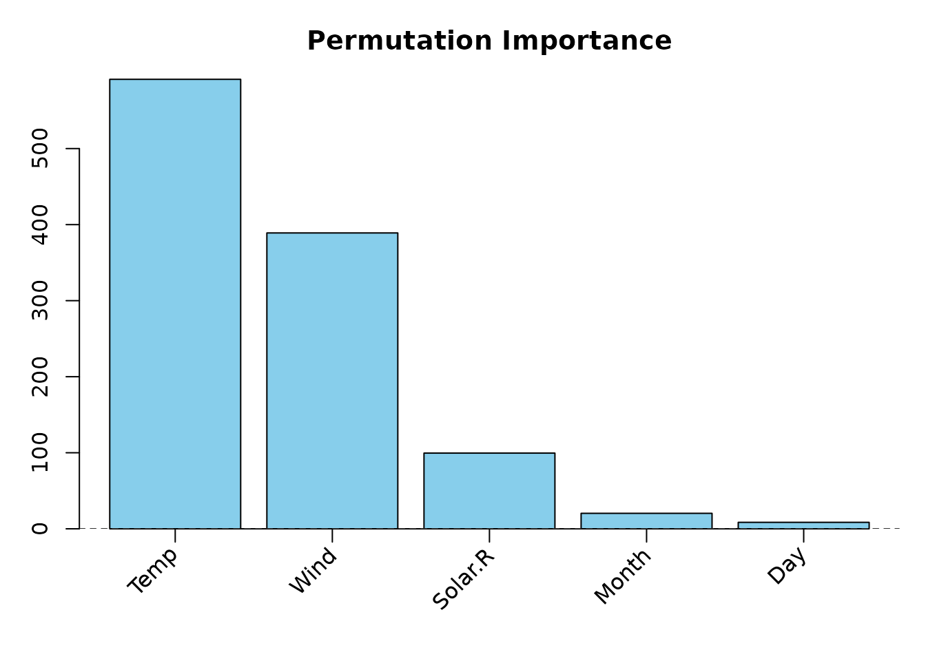

## barplot with visualization of the distribution: an
## interval between the .25 and .75 quantiles of the per 
## Tree values is added to the plot
plot(PI_permimp500, type = "bar", interval = "quantile")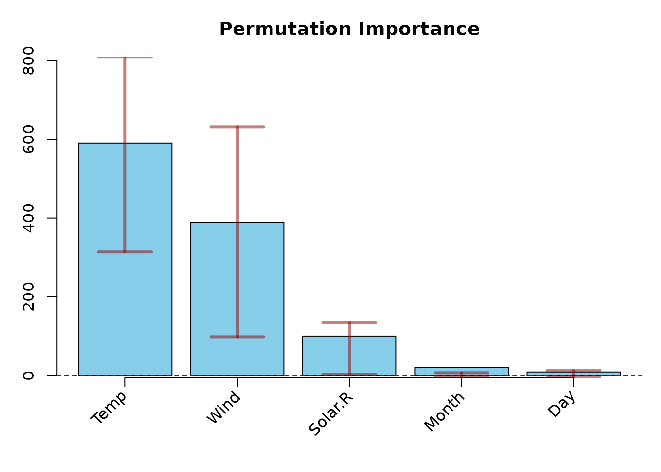

## horizontal boxplot
plot(PI_permimp500, type = "box", horizontal = TRUE)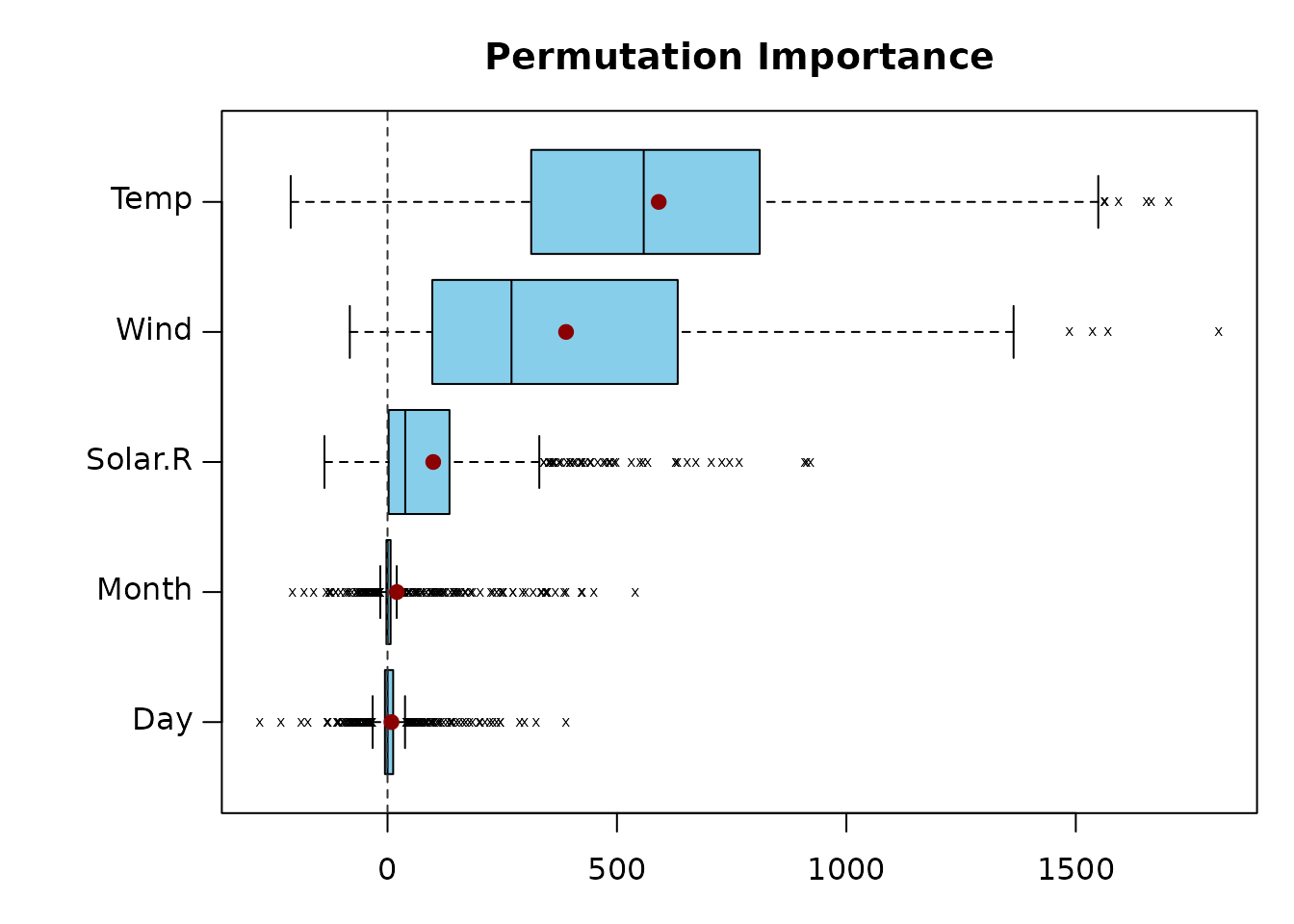

## unsorted-dotplot
plot(PI_permimp500, type = "dot", sort = FALSE, 
     interval = "quantile")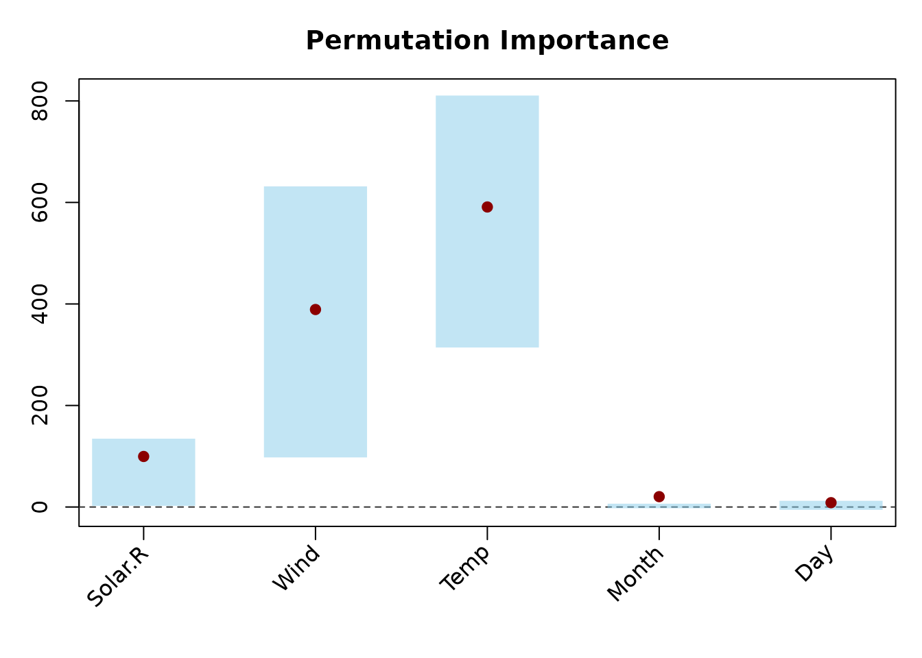

Additionally you can:

• Use your favorite colors with arguments col and intervalColor.
• Use different a quantile interval with intervalProbs = c(<lower_quantile>, <upper_quantile>).³
• Choose your own title the title with main
• Modify the margin with margin.

Although we would advise against this in most situations, you can also:

• Plot only the <integer value> predictors with the highest values with nVar = <integer value>.
  
• Visualize the distribution using the standard deviation of the perTree values with interval = "sd". This is almost always a bad idea, because it falsely suggests that the distribution is symmetric. Please don’t use this option.

For more detailed information check ?plot.VarImp.

B.2. Other VarImp-methods

(Currently) there are three more VarImp-methods:

• print: prints the $values
• ranks: prints the (reverse) rankings of the $values
• subset: creates a subset that is itself also aVarImp-object. Only to be used in very limited settings, and when you know what you are doing.

Other related functions are:

• as.VarImp: creates a VarImp-object from a matrix/data.frame of perTree values, or from a numerical vector of importance values.
• is.VarImp: checks if an object is of the VarImp-class.

C. permimp applied to randomForest-objects

As mentioned in the introduction, the permimp-package can also deal with with random forests that were grown using the randomForest-package Liaw and Wiener (2002), which applies the original tree growing algorithm based on impurity reduction Breiman (2001).

Let’s first grow a (small) forest.

library("randomForest", quietly = TRUE)
#> randomForest 4.7-1.2
#> Type rfNews() to see new features/changes/bug fixes.
set.seed(542863)
rfAirq50 <- randomForest(Ozone ~ ., data = airq, mtry = 2, replace = FALSE, 
                         nodesize = 7, keep.forest = TRUE, keep.inbag = TRUE)

Note that keep.forest = TRUE and keep.inbag = TRUE. The permimp-function requires information about which observations were in-bag (IB) or out-of-bag (OOB), as well as information about the split points in each tree. Without this information, the (Conditional) Permutation Importance algorithm cannot be executed.

CPI_permimpRF <- permimp(rfAirq50, conditional = TRUE, progressBar = FALSE)
plot(CPI_permimpRF, horizontal = TRUE)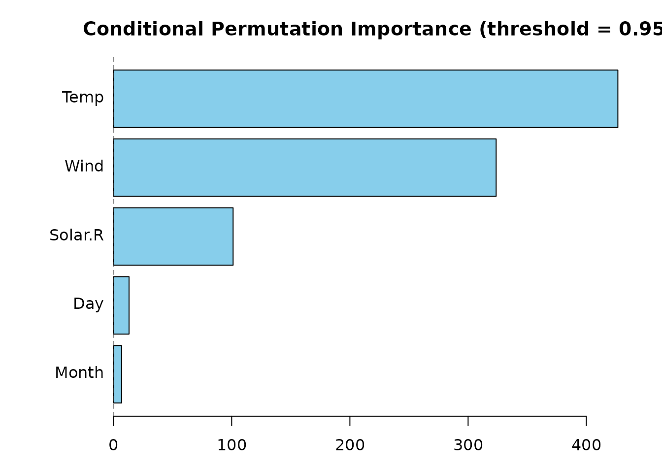

When calling permimp for a randomForest object form the randomForest-package, a menu is prompted that ask whether you are sure that the data-objects used to fit the random forest have not changed. This is because the permimp computations rely on those data-objects, and automatically search for them in the environment. If these data-objects have changed, the permimp results can be distorted.

---

Part II: New Conditional Permutation Implementation

This part explains the new implementation of the conditional permutation importance, and discusses the differences with the original implementation in party, as described by Strobl et al. (2008). First the the idea behind the conditional implementation is briefly recapitulated, followed by a discussion of the original implementation. Then the new implementation is explained, and the main differences with the original are emphasized. Finally, some practical implications of the new implementation are given, and the interpretation and possible use of the threshold value are discussed.

A. Recapitulation: Conditional Permutation Importance.

A researcher may be interested in whether a predictor $X$ and the outcome $Y$ are independent. The “null-hypothesis” is then $P(Y | X) = P(Y)$. This corresponds with the unconditional permutation importance. When $X$ and $Y$ are indeed independent, permuting $X$ should not significantly change the prediction accuracy of the tree/forest. The expected permutation importance value is zero.

However, a researcher may also be interested in the conditional independence of $X$ and $Y$, conditionally on the values of some other predictors $Z$. The “null-hypothesis” is then $P(Y | X, Z) = P(Y | Z)$. Rather than “completely” permuting the $X$ values, the $X$ values can be permuted conditionally, given their corresponding $Z$ values. This corresponds to the conditional permutation scheme. When $X$ and $Y$ are conditionally independent, ideally, a conditional importance measure should be zero.

If $X$ and $Z$ are independent, both permutation schemes will give the same results. Or in practice, similar importance values. Yet a dependence between $X$ and $Z$ will result in differences between the unconditional and the conditional permutation schemes, and the corresponding importance values.

Strobl et al. (2008) proposed to specify a partitioning (grid) of the predictor space based on $Z$ (for each tree), in order to (conditionally) permute the values of $X$ withing each partition (i.e., cell in the grid). According to Strobl et al. (2008) this partitioning should (1) be applicable to variables of all types; (2) be as parsimonious as possible, but (3) be also computationally feasible. Therefore they suggested to define the partitioning grid for each tree by means of the partitions of the predictor space induced by that tree. More precisely, using all the split points for $Z$ in the tree, $Z$ is discretized and the complete predictor space is partitioned using the discretized $Z$.

Note that this partitioning does not correspond with the recursive partitioning of a tree. In a tree only the top node splits the complete predictor space, all the following splits are conditional on the parent nodes. In contrast, for the conditional permutation grid, all the split points split the complete predictor space, which leads to a more fine-grained grid.

In practice, the number of observations is finite. In situation with a relatively low number of observations, the grid for the conditional permutation may become to fine grained, making conditionally permuting practically infeasible. Therefore, the selection of $Z$ (the predictors to condition on) is not a sinecure.

B. Original Implementation (party::varimp)

In their original implementation (cf, party::varimp), Strobl et al. (2008) argued to only include those variables in $Z$ whose empirical correlation with $X$ exceeds a certain moderate threshold. For continuous variables the Pearson correlation could be used, but for the general case they proposed to use the conditional inference framework promoted by Hothorn, Hornik, and Zeileis (2006). Applying this framework provides p-values, which have the advantage that they are comparable for variables of all types, and that they can serve as an intuitive and objective means of selecting the variables Z to condition on.

The original implementation can be described as follows:

For every predictor $X$

1. Test which other predictors are related to $X$, applying the conditional inference framework (Hothorn et al. 2006) using the full data/training set.
2. Only include those other predictors in $Z$ for which the $p$-value of the test is smaller than (1 - threshold).
3. Within each tree:
   1. Gather all the split points for every predictor in $Z$.
   2. Discretize the predictors in $Z$ using the gathered split points, and create a partitioning of the predictor space.
   3. Within each partition, permute the values of predictor $X$.

Some issues

There are, however, two important issues with this implementation:

1. For (some of) the tests in the conditional inference framework, the $p$-values not only depend on the strength of the (cor)relation, but also on the sample size. For instance, in big samples small correlations can also lead to small $p$-values.
2. (Some of the tests in) the conditional inference framework only test for linear dependence. For instance, for continuous variables a correlation test is used. Of course, dependence between variables is not limited to linear dependence. As a result, when $X$ and $W$ are continuous and have a U-shaped independence structure, $W$ will not be included in $Z$.

C. New Implementation (permimp).

The new implementation tries to mitigate the two issues raised above, by taking advantage of the fact that within each tree not the original values of the predictors, but only the partitions are important for the prediction of the outcome. That is, one can argue that the tree-based partitioning rather than the original values should be used to decide which other predictors should be included in $Z$. Applying this rationale, the new implementation can be described as follows:

In every tree, for every predictor with splits in the tree:

1. Discretize the in-bag values for each predictor using the split points: $X$ => $X_d$.

2. For every discretized $X_d$:

   1. Test which other discretized predictors $W_d$ are related to $X_d$, applying a $\chi^2$-independence tests (using only the in-bag values).
   2. Only include those other predictors $W$ in $Z$ for which the $p$-value of the test is smaller than (1 - threshold).
   3. Create the partitioning of the predictor space using the discretized $Z$.
   4. Within each partition, permute the values of predictor $X$.

Important implications

The $\chi^2$-independence test does not (directly) depend on sample size. Therefore, the new implementation is less sensitive to the number of observations. In addition, the $\chi^2$-independence test is not limited to linear dependence. Hence, the new implementation mitigates the two issue raised above. Because of this, the threshold-value is easier to use and interpret (see below).

Under the new implementation it is possible that $Z$ differs across trees. Yet this is also the case under the original implementation, since not all predictors in $Z$ are used as splitting variable in each tree. In addition, due to the randomness in random forests (subsampling/bootstrapping and mtry selection), it is very unlikely that there are two trees in the forest with exactly the same splitting points. Therefore, the conditional sampling scheme almost surely differs across trees.

D. How to Use the Threshold.

The threshold-value can be interpreted as a tuning parameter to make the permutation more or less conditional. A threshold = 0 and a threshold = 1 corresponding to permuting as conditional as possible and permuting completely unconditional, respectively. A threshold = .95, the default in permimp, only includes those $W$ in $Z$ for which $W_d$ and $X_d$ are dependent (with $\alpha$-level = .05).

Yet threshold values smaller than threshold = .5 generally make the selection of the predictors to condition on too greedy, without a meaningful impact on the CPI pattern. Therefore, we recommend using threshold values between .5 and 1.

Some research questions are best answered with a more marginal importance measure, while other questions are better answered using a more partial importance measure. In many situations, however, it is not clear which measure best fits the research question. Therefore, we argue that in these cases it can be interesting to evaluate the importance (rankings) of the predictors for different threshold-values. This strategy can provide more insight in how the conditioning affects the permutation importance values.

In the original implementation, setting a sensible threshold proved to be hard, because the practical meaning of the threshold depended on the sample size and on the type of variables (cf. the issues raised above). In the new implementation, the threshold’s interpretation is clearer and more stable. In addition, the simulation studies by Debeer and Strobl (2020) suggest that the new implementation (a) allows a more gradual shift from unconditional to conditional; and (b) gives more stable importance measure computations.

As an additional feature, the permimp can provide some diagnostics about the conditional permutation. When thresholdDiagnostics = TRUE, the permimp-function monitors whether or not a conditional permutation scheme was feasible for each predictor $X$ in each tree. This information is translated in messages that suggest to either or decrease the threshold.

First, it is possible that the conditioning grid is so fine-grained that permuting $X$ conditionally cannot lead to observations ending up in a different end-node of the tree. In other words, the prediction accuracy before and after permuting will be always equal. If this issue occurs in more than 50 percent of the trees that include $X$ as a splitting variable, permimp will produce a note, and suggest to increase the threshold-value. A higher threshold-value may result in a less fine-grained partitioning, making the conditional permutation feasible again.

Second, it is possible that there are no $W$ in the tree for which the $\chi^2$-independence test between $W_d$ and $X_d$ is smaller than (1 - threshold). This implies $Z$ will be an empty set, and conditionally permuting is impossible. That is, without a partitioning/grid, it is equal to unconditionally permuting. If this issue occurs in more than 50 percent of the trees that include $X$ as a splitting variable, permimp will produce a note, and suggest to decrease the threshold-value. A lower threshold-value includes more $W$ in $Z$, making the conditional permutation feasible again.

References

Breiman, Leo. 2001. “Random Forests.” Machine Learning 45 (1): 5–32. https://doi.org/10.1023/a:1010933404324.

Debeer, Dries, and Carolin Strobl. 2020. “Conditional Permuation Importance Revisited.”

Hothorn, Torsten, Kurt Hornik, Mark A van de Wiel, and Achim Zeileis. 2006. “A Lego System for Conditional Inference.” The American Statistician 60 (August). https://doi.org/https://doi.org/10.1198/000313006X118430.

Hothorn, Torsten, Kurt Hornik, and Achim Zeileis. 2006. “Unbiased Recursive Partitioning: A Conditional Inference Framework.” Journal of Computational and Graphical Statistics 15 (3): 651–74. https://doi.org/10.1198/106186006x133933.

Liaw, Andy, and Matthew Wiener. 2002. “Classification and Regression by randomForest.” R News 2 (3): 18–22. https://CRAN.R-project.org/doc/Rnews/.

Strobl, Carolin, Anne-Laure Boulesteix, Thomas Kneib, Thomas Augustin, and Achim Zeileis. 2008. “Conditional Variable Importance for Random Forests.” BMC Bioinformatics 9 (1): 307. https://doi.org/10.1186/1471-2105-9-307.